I learn robotics in industry

Sharing my recent learnings about fundamental robotics.

Robotics - Inverse kinematics [part 1]

As promised, I'll be talking about inverse kinematics this week. I never had a chance to dive into this topic during my PhD. Thanks to the many open-source packages (e.g., DART, MATLAB robotics toolbox), many students do not need to actually implement an inverse kinematics solver when they study robotics. Recently at work, I was able to spend more time reading about inverse kinematics. (I'm actually grateful for this chance to use work time to fill in some gaps in my knowledge.)

From a controls point of view, robotic application is about how we "move (action)" the robot to "do (result)" tasks we desire. Robots have joints that allow their links, i.e., the robot body, to move. The desired tasks are often done by the end-effector, i.e., the robotic hand. The subject of understanding how each joint movement affects the end-effector movement is called forward kinematics (action → result). The reverse is then called inverse kinematics (IK), which talks about finding the joint angles that put the end-effector at the right location (result → action).

The main challenge about IK is that there is no guarantee we can find an action for the joints based on the result we want to get for the end-effector. Sometimes IK solvers fail because the action does not exist, meaning that there are certain places that the end-effector cannot reach. However, there are also cases when there exist an action to achieve the result but we didn’t find it! Therefore, designing a robust IK solve is both hard and important for engineers to make the robot work efficiently.

(Jumping from here to the next section requires 5 chapters worth of robotics knowledge. So don’t feel discouraged if you find it hard to understand.)

When it comes to solving a problem, we might think of writing down some equations and solve for an exact solution like what we do with linear algebra. However, this is not always doable for solving IK problem. In stead, we will talk about one popular method - Numerical inverse kinematics using Newton-Raphson method.

Here is an example, consider we are finding the joint angles that can holds the end-effector at a desired (x,y,z) position, the IK process is as follows:

• we need to first understand the mapping from joint angles to the end-effector location. Does it sounds familiar? Right, this is the forward kinematics equation, denoted here as:

  

• IK is about finding the right joint angles that achieve the target end-effector location:

  

• The idea here is we want to build a process that help us to “iteratively find” the IK solution. In other words, we want the error equation to gradually become zero:

  

• Taking a closer look at the error function, we use Taylor expansion to get:

  

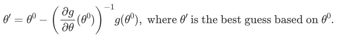
• This gives us an idea of what the best guess of a solution is (ignoring higher-order-terms):

  

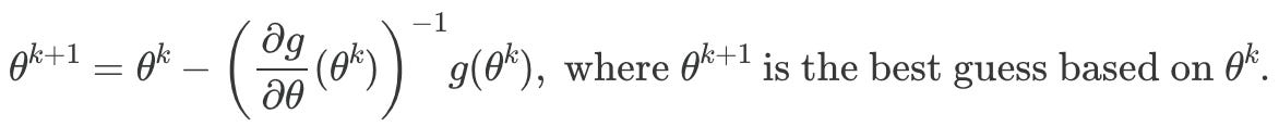
• This gives us an iterative function where we improve our solution and bring error function closer and closer to zero:

  

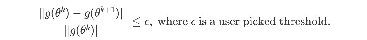
• Any iterative process needs a stopping criterion. In IK, we stop when the solver stops making progress:

  

  

Now we have some fundamentals about IK, next time, we will start looking at IK from a “velocity” point of view, which makes the formulation more generalizable.

(Haha, didn’t expect this to be this long. See you next week!)